A safety function only earns its SIL when the numbers say so, and that number is the average probability of failure on demand. This guide walks through the simplified formulas, a solved trip example and the field factors that quietly push a design out of its band.
PFDavg tells you how likely a safety function is to be dead when the process needs it. Here we work through the 1oo1, 1oo2 and 2oo3 formulas with real numbers and show how proof testing and common cause change the answer.
What Is PFDavg Calculation?
PFDavg calculation finds the average probability that a safety instrumented function will fail to act on demand, averaged over its proof test interval. For a single channel the simplified answer is PFDavg = λDU × TI ÷ 2, and that result decides which SIL band the function can claim.
- 1oo1: PFDavg = λDU × TI ÷ 2
- 1oo2: PFDavg = (λDU × TI)² ÷ 3 + β × λDU × TI ÷ 2
- 2oo3: PFDavg = (λDU × TI)² + β × λDU × TI ÷ 2
- SIL 1 = 0.01 to 0.1, SIL 2 = 0.001 to 0.01, SIL 3 = 0.0001 to 0.001
- Risk reduction factor RRF = 1 ÷ PFDavg, so SIL 2 needs RRF above 100
In the IEC 61511 lifecycle, PFDavg calculation sits inside the SIL verification step, where the designed loop is checked against the target from the hazard study. If the target itself is still unclear, start with our basics on what SIL means and come back to the numbers here.
Engineers in Indian refineries and fertiliser plants often meet PFD first in a vendor report. Once you can do a PFDavg calculation by hand, such reports become easy to check.
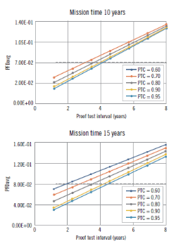
The Control Global graph plots PFDavg against proof test interval, and longer intervals let hidden failures sit longer.
PFDavg Formula for 1oo1, 1oo2 and 2oo3
λDU is the dangerous undetected failure rate per hour, taken from the FMEDA or the safety manual, and TI is the proof test interval in hours. Only undetected dangerous failures matter here, because detected ones are flagged by diagnostics, as explained in safe failure fraction.
1oo2: PFDavg = (λDU × TI)² ÷ 3 + β × λDU × TI ÷ 2
2oo3: PFDavg = (λDU × TI)² + β × λDU × TI ÷ 2
2oo2: PFDavg = λDU × TI
β = common cause fraction, 0.1 = 10 %
In the redundant formulas the squared term covers two independent failures, while the β term covers one shared cause that kills every channel at once. The voting logic itself is described in voting architectures for safety systems and in our note on 2oo3 voting logic.
These simplified equations in the style of IEC 61508 Part 6 ignore repair time, diagnostics and imperfect testing. Use them for a first PFDavg calculation, then confirm with the full method.
In most real 1oo2 designs the β term is larger than the independent squared term. That is why adding a second identical transmitter rarely gives the full tenfold gain people expect.
PFDavg Calculation Result and SIL Band Table
| SIL | PFDavg (low demand) | RRF | PFH per hour (high demand) |
|---|---|---|---|
| SIL 4 | 0.00001 to 0.0001 | 10,000 to 100,000 | 0.000000001 to 0.00000001 |
| SIL 3 | 0.0001 to 0.001 | 1,000 to 10,000 | 0.00000001 to 0.0000001 |
| SIL 2 | 0.001 to 0.01 | 100 to 1,000 | 0.0000001 to 0.000001 |
| SIL 1 | 0.01 to 0.1 | 10 to 100 | 0.000001 to 0.00001 |
The same table appears in the 61508 Association workshop on SIL calculations by Ian Dolan of Sella Controls. Low demand mode uses PFDavg, while a function demanded more than once a year uses PFH, and the target band normally comes from a LOPA study.
Step by Step PFDavg Calculation Method
The final element usually carries the largest share, so look closely at the valve, actuator and solenoid data in SIS final element reliability. Sensors and a certified logic solver normally add a much smaller part of the PFDavg calculation.
Solved Example: PFDavg Calculation for a Pressure Trip
Take a high pressure trip where each transmitter has λDU = 2 per million hours, a one year proof test interval of 8760 hours and β of 10 percent. We run the PFDavg calculation for the sensor subsystem in all three architectures.
1oo1 = 0.01752 ÷ 2 = 0.00876
RRF = 114, SIL 2 band
Squared term = 0.01752² ÷ 3 = 0.000102
β term = 0.1 × 0.01752 ÷ 2 = 0.000876
1oo2 = 0.000978, RRF 1022, SIL 3 band
2oo3 = 0.000307 + 0.000876 = 0.00118
RRF 845, SIL 2 band
The single transmitter sits in SIL 2, while 1oo2 just crosses into the SIL 3 band. 2oo3 is slightly worse than 1oo2 on PFD, but it trips falsely far less often, which is why many furnace and compressor trips still use it.
The β term of 0.000876 is about 90 percent of the 1oo2 PFDavg calculation result, so halving β helps far more than a better transmitter.
PFDavg Calculator for 1oo1, 1oo2 and 2oo3
This PFDavg calculation tool uses the simplified formulas for quick checks and student practice. Repair time, diagnostics and imperfect testing are added by hand in the next sections.
Always state the λDU unit on your calculation sheet, because vendors quote per hour, per year or in FIT. One FIT is one failure per billion hours, so 2000 FIT equals 2 per million hours.
How Proof Test Interval Changes PFDavg
For a 1oo1 channel PFDavg rises in a straight line with TI, so doubling the interval doubles the result. The table uses λDU = 2 per million hours, the same transmitter as the solved example, and our article on proof test interval and coverage covers how to plan the tests.
| Proof Test Interval | 1oo1 PFDavg | RRF | Band |
|---|---|---|---|
| 6 months | 0.00438 | 228 | SIL 2 |
| 1 year | 0.00876 | 114 | SIL 2 |
| 2 years | 0.01752 | 57 | SIL 1 |
| 3 years | 0.02628 | 38 | SIL 1 |
| 4 years | 0.03504 | 29 | SIL 1 |
Control Global author Bill Mostia notes that, in his example, the SIL 1 limit can be exceeded once the proof test interval passes about three to four years. That is a real risk when a plant stretches tests to match a four or five year turnaround cycle.
If the turnaround cannot be shortened, online tests can help. Partial stroke testing of ESD valves catches part of the valve failures between full tests and lowers the effective λDU in the PFDavg calculation.
Proof Test Coverage and Mission Time
Real proof tests never find every hidden failure, and Bill Mostia defines proof test coverage as the fraction of dangerous undetected failures a user test can detect. He also notes that 100 percent coverage was long assumed, while good practice aims for typically greater than 95 percent.
PTC = 0.9, TI = 8760 h, MT = 15 years = 131400 h
Tested part = 0.9 × 0.00876 = 0.00788
Untested part = 0.1 × 0.000002 × 131400 ÷ 2 = 0.01314
PFDavg ≈ 0.0210, SIL 1 band
The untested 10 percent stays hidden for the whole mission time, so a transmitter that looked SIL 2 in the simple PFDavg calculation drops to SIL 1.
The 61508 Association workshop shows the same effect at system level. With a valve test coverage of 85 percent and the β multipliers applied, the example total moves from 0.00129 to 0.00339, and the RRF falls from 777 to 295.
The mission time in this formula is the time until the device is fully overhauled or replaced to an as new condition. It is often tied to the planned device or plant life, so it must be written in the safety requirements specification.
Common Cause Beta Factor in PFDavg Calculation
Common cause failures hit redundant channels together, for example a shared plugged impulse tap, wrong calibration by the same technician or a single power supply. exida, in a blog by Dr Steve Gandy, defines the common cause rate as λcc = β × λ.
Gandy quotes IEC 61508 Part 6 ranges of 0.005 to 0.05 for programmable electronics and 0.01 to 0.1 for field equipment. He adds that the exSILentia tool uses 10 percent as its default when no better data exists.
| β for 1oo2 | Squared Term | β Term | 1oo2 PFDavg |
|---|---|---|---|
| 2 % | 0.000102 | 0.000175 | 0.000277 |
| 5 % | 0.000102 | 0.000438 | 0.000540 |
| 10 % | 0.000102 | 0.000876 | 0.000978 |
Cutting β from 10 to 2 percent improves this 1oo2 PFDavg calculation about three and a half times, a gain no transmitter upgrade can match.
Use separate process taps, separate impulse lines and if possible two different measuring principles for redundant trip sensors. Stagger calibration so one technician error cannot reach both channels on the same day.
Choosing 1oo1, 1oo2 or 2oo3 for a Safety Loop
One channel, any failure to act is a failure on demand and any safe fault trips the plant.
Either of two channels can trip, so dangerous failures are covered but false trips double.
Any two of three channels must agree, giving low PFD and high availability together.
Architecture choice is not only about PFD, since a nuisance trip on a cracker or boiler has its own safety and cost penalty. Our page on the emergency shutdown system shows how these votes are built in a real ESD, and SIS and BPCS differences explains why sensors must stay independent.
Common PFDavg Calculation Mistakes and Field Fixes
| Symptom | Likely Cause | Fix |
|---|---|---|
| Result looks too good | λD used instead of λDU | Take only the dangerous undetected rate |
| SIL 3 from two cheap sensors | β set to zero | Use 5 to 10 percent unless data proves less |
| Valve dominates total | Long test interval, low coverage | Add partial stroke tests, shorten TI |
| Paper SIL never matches site | Tests not done on schedule | Track actual test dates in the CMMS |
- λDU taken from a certified FMEDA or proven in use data, with units stated.
- Proof test interval matches the actual turnaround and maintenance plan.
- Proof test coverage and mission time entered for every device.
- β chosen for each redundant group and justified in writing.
- Architectural constraints and systematic capability also checked.
- Quick hand check of vendor reports.
- Shows which term dominates.
- Easy to audit in a spreadsheet.
- Ignore repair time and diagnostics.
- Assume perfect proof testing.
- Optimistic for long mission times.
exida warns that simplified equations can omit variables and give an optimistic result. In its example, two sets of variables gave a full SIL level of difference in the PFDavg calculation.
PFDavg Calculation Is Only Half of SIL Verification
A good PFDavg calculation is not enough, since the loop must also meet hardware fault tolerance and systematic capability limits. Verification checks the design on paper, while validation proves it on site, a difference covered in SIL verification vs SIL validation.
Feed each PFDavg calculation back into the SIF design before purchase orders are placed, because changes after FAT cost far more.
61508 Association SIL Calculations Workshop PDF
Video: It Is All About PFDavg
PFDavg Calculation FAQ
For one channel, multiply the dangerous undetected failure rate per hour by the proof test interval in hours and divide by 2. For redundant channels, use the 1oo2 or 2oo3 formula with a common cause term.
Calculate the sensors, logic solver and final elements separately. Then add them to get the total for the safety function.
A SIL 2 function in low demand mode needs a PFDavg from 0.001 up to below 0.01. That equals a risk reduction factor above 100 and up to 1000.
The value must cover the whole loop, not one device. Hardware fault tolerance and systematic capability must also meet the SIL 2 rules of the standard.
PFD is the probability of being failed at a given moment, and it rises after each proof test until the next one. It looks like a sawtooth over the life of the device.
PFDavg is the average of that sawtooth over the test interval. It is the single number used to compare a function against its target band.
For a single channel PFDavg rises in direct proportion to the test interval. Doubling the interval from one to two years doubles the average probability of failure.
In redundant systems the effect is even stronger for the squared term. Long turnarounds are a common reason why a design slips from one band to the next.
Beta is the fraction of failures that strike all redundant channels at the same time from one shared cause. Typical values range from 1 to 10 percent for field devices.
A value of 10 percent is a common default when no better data is available. Separate taps, diverse sensors and staggered testing are the usual ways to lower it.
Yes, the simplified formulas work well in a spreadsheet and are ideal for quick checks, training and comparing several designs. Keep every rate in per hour units and every time in hours.
For a formal report, use full equations with repair time and test coverage. Many companies use validated tools such as exSILentia for that final step.
Related Articles
- SIL Verification
- What Is SIL Safety Integrity Level
- Proof Test Interval and Coverage for Safety Transmitters
- Voting Architectures in Safety Systems
- SIS Final Element Reliability
External References
- SIL Calculations and Use of IEC 61508 Part 6, 61508 Association
- SIS: How Testing Impacts Reliability, Control Global
- Safety Integrity Level, Wikipedia
What We Learn Today
- PFDavg calculation for one channel is λDU × TI ÷ 2, and the result maps directly to a SIL band and a risk reduction factor.
- In redundant 1oo2 and 2oo3 designs the common cause beta term usually dominates, so independence and diversity matter more than device brand.
- Long proof test intervals, low test coverage and long mission times can push a SIL 2 loop into SIL 1 without any visible change.