When a compressor trips, the control room may see hundreds of alarms in a few minutes, and the first real cause is buried somewhere in that flood. Data driven methods can rank the likely starting point in minutes, so engineers spend their time fixing the fault instead of searching for it.
Process upsets leave a detailed trail in the historian and the alarm and event journal. Machine learning and causal analysis read that trail to point engineers toward the most likely first cause of a trip or alarm flood.
What Is AI Root Cause Analysis?
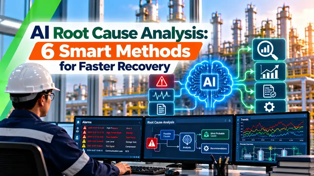
AI root cause analysis is the use of machine learning and statistical causal methods on process data, alarms and events to identify the most likely first cause of an upset, trip or alarm flood. It builds on the ideas in artificial intelligence and machine learning, but focuses on cause and effect, not just pattern spotting.
A classic investigation uses the 5 Whys, a fishbone diagram or a fault tree, led by experienced engineers. Data driven tools do not replace that thinking, but they shrink the list of suspects from hundreds of tags to a handful.

The raw material for AI root cause analysis is data the plant already stores, such as trends in the process historian and the alarm and event journal of the DCS. The better the timestamps and tag names, the better the results.
Why Plants Need Data Driven Diagnosis
ABB Review describes an upstream oil and gas system that produced about 1.5 GB of compressed data every month, from more than 3900 tags and 250,000 alarms and events. No engineer can read that much by hand after every upset.
The same article notes that alarm floods have been linked to most of the chemical incidents investigated by the US Chemical Safety Board. Good alarm management to ISA 18.2 reduces floods, and causal tools help explain the ones that still happen.
In the ABB case study, a recurring flood class was traced to the produced water reinjection system, where the diagnosed root cause was a change of fuel type in the pumps. A low flow alarm on one pump was followed by a second pump, a double trip and high level alarms in a degassing drum.
6 Smart Methods Behind AI Root Cause Analysis
Tests whether the past of one signal improves the prediction of another.
Measures directed information flow between signals, including nonlinear links.
A directed graph of causes with probabilities that update with evidence.
Finds alarm orders that repeat across many upsets.
Groups similar alarm floods so one diagnosis covers a whole class.
Neural networks trained on labelled alarm sequences of known faults.
Granger causality, as Zhang, Hu and Gopaluni explain, compares the error of a model with and without the past of a candidate cause, using linear vector autoregression. It works on continuous data, so alarm events need other methods such as point process models or transfer entropy.
Bayesian networks are useful because they can start from the plant topology and the knowledge of operators, then update with data. Many tools also add correlation views and the outlier scores described in anomaly detection with machine learning.
Check the clock sync between the DCS, PLCs and historian before any causal study. A 2 second offset between systems can make an effect appear before its cause and reverse the whole result.
Bayesian Root Cause Probability
A simple way to see Bayesian thinking is to compare two candidate causes for the same symptom. Each gets a prior probability from history and a likelihood, which is the chance of seeing the symptom if that cause is true.
Example, pump low flow alarm S:
Cause A, fuel or feed change: prior 30 %, likelihood 90 %
Cause B, flow transmitter fault: prior 70 %, likelihood 20 %
A term = 0.30 × 0.90 = 0.27
B term = 0.70 × 0.20 = 0.14
P(A given S) = 0.27 ÷ 0.41 = 65.9 %, P(B given S) = 34.1 %
Root Cause Probability Calculator
The transmitter fault looked more likely before the evidence, yet the symptom fits a process change far better. Real tools repeat this over many nodes and many alarms, which is why the graph structure matters so much.
Second Example: Alarm Sequence Confidence
Suppose your journal shows that alarm X, a pump low flow, occurred 50 times last year, and in 45 of those cases alarm Y, a drum high level, followed within 60 seconds. The confidence of the rule X then Y is 45 ÷ 50 = 90 percent.
If Y occurred 60 times in total, the reverse rule has a confidence of 45 ÷ 60 = 75 percent, so X is the better candidate as the earlier link in the chain. A first out alarm on the trip panel gives a similar answer for one trip, but mining finds patterns across hundreds of events.
How an AI Root Cause Analysis Workflow Runs
Data collection is easier when the tags follow a clear naming scheme, as described in SCADA tag database design. Historian compression settings also matter, because heavily compressed trends lose the small early changes that reveal the first cause.
Many sites run the analysis on a server near the PI or AVEVA historian rather than in the cloud, for both speed and security. The trade offs are similar to those in edge AI versus cloud AI.
Real Case Results From Research and Industry
In the ABB study of an offshore gas oil separation plant, 382 days of data were analysed with a flood threshold of 8 alarms per 10 minutes. The tool found 926 alarm floods involving 1473 unique alarm tags and grouped them automatically into 5 classes.
Javanbakht and co authors trained a deep learning model on the Tennessee Eastman benchmark, with 41 measured variables and 82 alarm tags. They reported test accuracy of 0.96 and identified every studied fault from the first five alarms.
Zhang, Hu and Gopaluni compared causal methods on alarm data and found that their neural point process approach reached 0.917 accuracy in 11.6 seconds. Transfer entropy on the same case reached 0.731 and took 492.8 seconds.
| Method | Data Needed | Strength | Weakness |
|---|---|---|---|
| Granger causality | Continuous trends | Simple, well tested statistics | Assumes linear links and steady data |
| Transfer entropy | Trends or binary alarms | Captures nonlinear links | Slow on long records |
| Bayesian network | Topology plus history | Uses expert knowledge | Graph must be built and kept current |
| Sequence mining | Alarm journal | Easy to explain | Order does not always mean cause |
| Deep learning | Labelled fault data | High accuracy on known faults | Needs labels, weak on new faults |
Limits You Must Respect
The arXiv authors note that labelled alarm data is hard to obtain, and their study used simulation data only. A model trained on known faults may also miss a failure mode it has never seen before.
Hidden variables are a common trap, such as ambient temperature affecting many loops at once or a sticky control valve shaking several flows. Pair the analysis with condition data, like the signals used in vibration analysis with AI, to see the full picture.
Keep a short written record of every confirmed root cause and link it to the alarm episode in the tool. These labels steadily improve future rankings and build a valuable plant knowledge base.
Starting AI Root Cause Analysis in an Indian Plant
- Historian and DCS clocks synchronised to one source.
- Alarm journal exported with tag, priority and timestamp.
- Known incidents listed with confirmed causes for testing.
- P&IDs or a tag topology available for the causal graph.
- Operators and process engineers involved in the review.
- Cybersecurity approval for any data leaving the control network.
- Shrinks hundreds of suspects to a few likely causes.
- Finds repeating patterns across many upsets.
- Uses historian data the plant already has.
- Supports HAZOP revalidation and alarm rationalisation.
- Results are only as good as the data quality.
- Correlation can be mistaken for cause.
- Deep learning needs labelled fault data.
- Needs engineering review and regular retraining.
Root cause findings often feed back into the HAZOP study revalidation and into control improvements such as model predictive control. They also help plan work in predictive and preventive maintenance programs.
Where This Approach Adds Most Value
Vendors now add these features to their platforms, as discussed in AI in PLC, SCADA and DCS. For a basic grounding in alarm types used in these studies, see 7 types of alarms in DCS.
Research Paper on Alarm Based Diagnosis
Video: Causal Inference in Engineering
AI Root Cause Analysis FAQ
It applies machine learning and causal statistics to historian trends and alarm journals after a process upset. The aim is to rank the most likely first cause of a trip or alarm flood.
It does not replace engineers or formal investigation methods. It shortens the search so that field checks start with the right equipment.
It tests whether the past values of one signal improve the prediction of another signal. If they do, the first signal is a candidate cause of the second.
The method suits continuous trends such as flow, pressure and level. It assumes fairly linear and steady behaviour, so results still need careful engineering judgement before any action on the plant.
You need historian trends, the alarm and event journal and a list of known trips with confirmed causes. Accurate time stamps across all systems are essential for reliable results.
A tag topology or simple P&ID connections makes the causal graph far better. Maintenance work orders and shift logs add valuable context for the review meeting with operators.
Yes, sequence mining, flood clustering and point process models work directly on alarm and event journals. ABB grouped 926 floods into 5 classes using alarm data in one study.
Adding process trends usually improves accuracy, because alarms are only threshold crossings. The trends show the small early changes in flow, pressure or temperature before any alarm appears.
Deep learning can be very accurate on faults it was trained on, such as the benchmark faults in academic studies. It needs many labelled examples, which most plants do not yet have.
Simpler causal methods are easier to explain to operators and auditors. Many sites start simple and add learning models as their labelled history grows.
Bad timestamps, compressed data and hidden variables can all point the analysis to the wrong tag. Correlation and the order of events do not always mean cause.
Process changes, new equipment and new product grades also make old models less accurate over time. Regular retraining and a strict engineering review keep the results trustworthy for operators.
Start with one unit that has frequent and costly trips, and audit its data quality first. Clean up chattering, stale and duplicate alarms before running any model.
Then test the tool against past incidents with known causes. Agreement with those cases builds trust among operators and managers before the tool is scaled to other units.
Related Articles
- Anomaly Detection With Machine Learning in Industry
- Alarm Management to ISA 18.2
- What Is a Process Historian
- AI in PLC, SCADA and DCS
- First Out Alarm PLC Logic
External References
- Alarm Based Root Cause Analysis in Industrial Processes Using Deep Learning, arXiv
- Unravelling Events and Alarms With Data Analytics Tools, ABB Review
- Granger Causality, Wikipedia
What We Learn Today
- AI root cause analysis ranks the likely first cause of a trip or alarm flood using historian trends, alarm journals and causal statistics, not guesswork.
- Granger causality suits continuous trends, while Bayesian networks, sequence mining and point process models handle alarms and expert knowledge better.
- Results depend on clean timestamps and good alarm data, and every ranked cause still needs confirmation by engineers and operators in the field.