
Every real-world signal, a voice, a temperature, a vibration, is smooth and continuous, yet every digital system can only ever store 0s and 1s. Here is exactly how that gap gets bridged, with live interactive charts you can adjust yourself, built right into this page.
What is Analog to Digital Conversion?
Analog to digital conversion is the process of transforming a continuous, infinitely variable signal into a discrete sequence of numbers that a digital system can store, process, and transmit.
An analog signal can take on any value at any instant, exactly like a dimmer switch smoothly fading a light. A digital signal, by contrast, only ever holds one of a fixed number of distinct values at each moment, more like a bank of separate on/off switches. Converting between the two is the foundation this guide builds on, and it directly complements our deep dive into ADC working principle, SNR, and ENOB, which covers the electronics of a single ADC chip rather than the broader family of conversion techniques covered here.
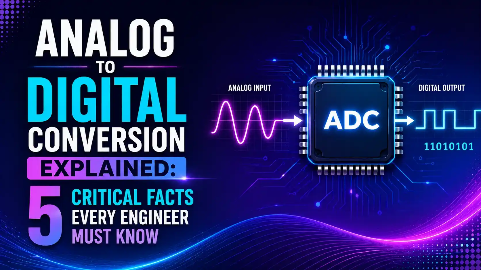
This guide covers the five critical facts behind analog to digital conversion, walking through pulse code modulation's three stages, delta modulation, and adaptive delta modulation, each shown with a live chart you can adjust directly on this page.
The Three Stages of Pulse Code Modulation
Pulse code modulation, or PCM, is the most widely used conversion technique, and it always follows the same three-stage sequence.
Sampling
The continuous signal's amplitude is measured at regular, discrete instants in time.
Quantization
Each sampled amplitude is rounded to the nearest of a fixed set of allowed levels.
Encoding
Each quantized level is assigned its own binary code, producing the final digital output.
5 Critical Facts About Analog to Digital Conversion
These five facts explain almost everything a working engineer needs to know about how conversion techniques actually behave.
Each PCM Stage Introduces Its Own Limitation
Sampling limits how fast the signal can change and still be captured, quantization limits how precisely each value is recorded, and encoding limits how compactly that value gets transmitted. A weakness in any one stage cannot be fixed by the others.
The Nyquist Theorem Sets a Hard Minimum Sampling Rate
The sampling rate must be at least twice the highest frequency present in the signal, Fs ≥ 2fmax. Sampling any slower causes aliasing, where higher frequencies fold back and masquerade as false lower frequencies that cannot be removed afterward.
Real Hardware Uses Flat-Top Sampling, Not Ideal Sampling
Ideal sampling would capture an instantaneous, zero-width value, which no real circuit can do. Practical ADCs use a sample-and-hold circuit instead, holding each captured value flat for a short duration while quantization and encoding catch up.
Quantization Error Can Never Be Fully Eliminated
Rounding a continuous amplitude to one of a finite set of levels always leaves a small residual error. That error only shrinks as more quantization levels are added, it never disappears entirely.
Delta Modulation Trades Resolution for Radical Simplicity
Rather than encoding each sample's full amplitude, delta modulation encodes only whether the signal moved up or down since the last sample, just one bit per sample. That simplicity comes at the cost of struggling to track signals that change too quickly.
Natural Sampling vs Flat-Top Sampling
Here is a live-drawn comparison of the two practical sampling methods, both capturing the exact same underlying analog waveform.
What is happening: In natural sampling, each pulse still traces the shape of the original waveform during its brief window. In flat-top sampling, the value at the leading edge of each pulse gets held flat for its entire duration.
A real example: A sample-and-hold circuit inside a practical ADC charges a small capacitor to the instantaneous signal voltage, then holds that charge steady while the rest of the conversion happens, producing exactly the flat-top behavior shown above.
Why it works: Quantization and encoding both take a small but nonzero amount of time to complete, so the sampled value needs to stay perfectly still during that window, which is precisely the job flat-top sampling performs.
The Nyquist Sampling Rate
Undersampling a signal does not just lose detail, it actively creates false frequencies that cannot be removed after the fact.
Nyquist minimum sampling rate: Fs ≥ 2 × fmax
Worked example: a signal contains frequencies up to 4 kHz
Minimum sampling rate: Fs = 2 × 4,000 = 8,000 samples per second
Quantization: Dividing the Signal Into Levels
Quantization takes the sampled amplitude and rounds it to the nearest of L available levels, each spanning a step size d.
Try It: Delta Modulation Slope Tracker
Adjust the step size to see how the staircase approximation either tracks the signal cleanly or falls behind during steep sections, a failure called slope overload.
Delta Modulation vs Adaptive Delta Modulation
Delta Modulation
Uses one fixed step size for every comparison. Simple to build, but a single step size is always a compromise between tracking steep signal sections and staying quiet during flat ones.
Adaptive Delta Modulation
Automatically grows the step size during steep sections to avoid slope overload, then shrinks it again during flatter sections to reduce granular noise.
What is happening: Standard delta modulation must pick one step size for the entire signal. Too small, and steep sections cause slope overload. Too large, and flat sections pick up unnecessary granular noise as the staircase hunts around the true value.
A real example: Adaptive delta modulation might double its step size for several consecutive samples all moving the same direction, correctly inferring a steep section is underway, then shrink back down once the signal levels off.
Why it works: By tying the step size to the signal's own recent behavior rather than fixing it in advance, adaptive delta modulation gets the tracking benefits of a large step size and the low noise benefits of a small one, without permanently committing to either.
PCM vs Delta Modulation vs Adaptive Delta Modulation
| Feature | PCM | Delta Modulation | Adaptive Delta Modulation |
|---|---|---|---|
| Bits per Sample | Multiple (n = log2 L) | 1 | 1 |
| Encodes | Full amplitude value | Direction of change only | Direction of change only |
| Circuit Complexity | Highest | Lowest | Moderate |
| Weakness | Bandwidth grows with resolution | Slope overload on fast signals | More complex step-size logic |
Where These Techniques Show Up
Voice and Audio Digitization
PCM underlies telephone systems, digital audio, and voice-over-IP encoding.
Low-Bandwidth Telemetry
Delta modulation's simple 1-bit stream suits bandwidth-constrained sensor links.
Instrumentation and Data Acquisition
Precision measurement systems rely on well-chosen sampling rates to avoid aliasing, the same reasoning behind proper RTD wiring and sensor signal integrity.
Advantages and Limitations of These Conversion Techniques
Why These Techniques Remain Essential
Limitations to Keep in Mind
Download Analog to Digital Conversion References
These two university lecture references go deeper into pulse code modulation and delta modulation.
Lecture 13: Pulse Code Modulation
Stanford University EE179 lecture notes on PCM and delta modulation
Lecture 11: Pulse Code Modulation, ELG3175
University of Ottawa lecture notes on sampling, quantization, and bandwidth
Watch: Pulse Code Modulation Explained
This video walks through the PCM process, covering sampling and quantization step by step.
FAQs on Analog to Digital Conversion
External References
- Stanford University, EE179, Lecture 13, Pulse Code Modulation
- University of Ottawa, ELG3175, Lecture 11, Pulse Code Modulation
- YouTube, Pulse Code Modulation PCM, Basics, Block Diagram, Process, Sampling and Quantization
What we learn today
- Analog to digital conversion transforms a continuous signal into a discrete numeric sequence through sampling, quantization, and encoding.
- The Nyquist theorem requires sampling at least twice the highest frequency present, or aliasing introduces unrecoverable errors.
- Real hardware uses flat-top sampling via sample-and-hold circuits, not the theoretical instantaneous ideal sampling.
- Quantization error is a fundamental, unavoidable cost of representing a continuous value with a finite set of levels.
- Delta modulation trades PCM's resolution for radical simplicity, at the cost of potential slope overload on fast-changing signals.