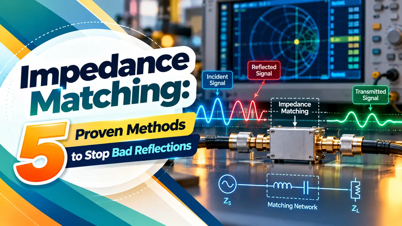
When a signal travels down a cable or PCB trace and meets a load of a different impedance, part of it bounces back toward the source. Impedance matching makes the load look like the line, so the signal is absorbed cleanly instead of echoing.
Impedance matching is about more than maximum power; at radio and fast digital frequencies it decides whether a signal arrives clean or full of reflections. This guide covers 50 and 75 Ω systems, VSWR, return loss, L networks, transformers and termination.
What Is Impedance Matching?
Impedance matching is the practice of making the impedance seen by a source equal to the impedance it is designed to drive, so that signal energy flows forward without bouncing back. If the term impedance is new to you, it is simply resistance plus reactance in an AC circuit.
At low frequencies and short wires the effect is small. Once a cable or trace becomes a noticeable fraction of a wavelength, every change in impedance along the path acts like a partial mirror for the travelling wave.
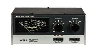
A VSWR meter like the one shown checks impedance matching between a transmitter and its antenna feed line. It compares forward and reflected power, and a reading close to 1.0 tells the operator that the antenna presents the right load.
Impedance Matching vs Maximum Power Transfer
Students first meet impedance matching through the maximum power transfer theorem, which says a source delivers the most power when the load resistance equals the source resistance. The source is modelled by its Thevenin equivalent, as shown in this guide to the Thevenin theorem.
With reactive parts, Analog Devices states the full condition in its Smith chart tutorial: the source impedance must equal the complex conjugate of the load, so RS plus jXS equals RL minus jXL. The reactances cancel and only the resistive parts share the power.
For signals and RF, impedance matching has a second and often more important job: stopping reflections on a transmission line. The same tutorial notes that this matters most at high frequencies, above about 100 MHz, where interconnects behave as lines rather than simple wires.
Analog Devices lists 50, 75, 100 and 600 Ω as common reference impedances. 600 Ω comes from old telephone and professional audio lines, long before RF coax existed.
Why 50 Ω and 75 Ω Became Standards
A coaxial cable has a characteristic impedance set by its conductor diameters and dielectric, not by its length. Everything RF explains that for air filled coax, about 30 Ω gives maximum peak power handling and about 77 Ω gives the lowest conductor loss.
50 Ω sits between these two and became the standard for RF equipment, test instruments and antennas. 75 Ω is used where low loss matters more than power, such as cable TV, video and the satellite dish cable running to a set top box.
Industrial networks follow the same logic. ControlNet uses 75 Ω coax with a 75 Ω termination resistor, while twisted pair buses like RS 485 use about 120 Ω.
Reflection Coefficient, VSWR and Return Loss
The reflection coefficient Γ is the ratio of reflected to incident voltage at the load. From it you get VSWR, the ratio of maximum to minimum voltage along the line, and return loss, how many decibels weaker the reflection is than the incident wave.
VSWR = (1 plus |Γ|) ÷ (1 minus |Γ|)
Return loss = minus 20 × log10 |Γ| dB
Reflected power = |Γ|² × 100 percent
Mismatch loss = minus 10 × log10 (1 minus |Γ|²) dB
Example: 75 Ω load on a 50 Ω line
Γ = (75 minus 50) ÷ (75 plus 50) = 25 ÷ 125 = 0.200
VSWR = 1.2 ÷ 0.8 = 1.50
Return loss = 20 × log10 (5) = 13.98 dB
Reflected power = 4.00 percent, mismatch loss = 0.177 dB
Everything RF quotes the same numbers for a 50 to 75 Ω junction: Γ of 0.20, 4 percent reflected power, about 14 dB return loss, VSWR of 1.5 and about 0.18 dB mismatch loss. Decibel arithmetic is explained in decibels in electronics.
Impedance Matching Calculator
| VSWR | |Γ| | Return Loss | Reflected Power |
|---|---|---|---|
| 1.1 | 0.048 | 26.4 dB | 0.23 percent |
| 1.5 | 0.200 | 14.0 dB | 4.0 percent |
| 2.0 | 0.333 | 9.5 dB | 11.1 percent |
| 3.0 | 0.500 | 6.0 dB | 25.0 percent |
Many antenna and RF module datasheets ask for VSWR below 2.0, about 11 percent reflected power. Good impedance matching on test ports and filters aims for 1.5 or better.
When Γ comes out negative, the load is below Z0 and the reflection is inverted. The size of Γ decides the loss, so VSWR and return loss use only its magnitude.
5 Impedance Matching Methods
One series and one shunt reactance transform a resistance up or down at one frequency.
Turns ratio changes impedance by the square of the ratio over a wide band.
A line section of impedance √(Z0 × ZL) and quarter wavelength long.
A resistor at the driver makes its output equal the trace impedance.
A resistor at the far end equal to Z0 absorbs the arriving wave.
Lumped L, pi and T networks use inductors and capacitors, whose reactance changes with frequency. That is why a lumped network gives a good match only over a limited band around its design frequency.
Designing an L Network for Impedance Matching
Second Worked Example: 50 Ω to 200 Ω at 100 MHz
Suppose a 50 Ω source must drive a 200 Ω resistive load at 100 MHz. Q = √(200 ÷ 50 minus 1) = √3 = 1.732, so the series reactance is 1.732 × 50 = 86.6 Ω and the shunt reactance is 200 ÷ 1.732 = 115.5 Ω.
In the low pass form, the series element is an inductor of 86.6 ÷ (2π × 100 MHz) = 137.8 nH, and the shunt element across the 200 Ω load is a capacitor of 1 ÷ (2π × 100 MHz × 115.5) = 13.78 pF. The nearest standard parts, about 140 nH and 13 pF plus trimming, complete the impedance matching network.
Analog Devices solves a similar 60 MHz impedance matching case on the Smith chart and notes that many component combinations give the same match, ignoring parasitics.
Every L network has a fixed Q set by the resistance ratio. If you need a wider or narrower bandwidth, a pi or T network adds a third element that lets you choose Q freely.
Transformer and Quarter Wave Impedance Matching
An ideal transformer reflects a load impedance to its primary multiplied by the square of the turns ratio. The voltage side of this rule is covered in transformer turns ratio, and the impedance rule follows directly from it.
For example, an old valve amplifier with an 800 Ω output needs a 10 to 1 transformer to drive an 8 Ω speaker, since 10 squared is 100. RF baluns use the same idea, with a 4 to 1 impedance balun turning a 300 Ω folded dipole into a 75 Ω feed.
A quarter wave transformer is a section of line with impedance equal to the geometric mean of the two impedances to be joined. Joining 50 Ω to 100 Ω needs a 70.7 Ω section exactly one quarter wavelength long at the operating frequency.
A quarter wave section is a quarter of the wavelength inside the cable or PCB, not in free space. Multiply the free space length by the velocity factor of the medium before cutting.
Termination for Digital Signals and Field Buses
Fast logic edges contain high frequency content even at a modest clock rate, so a long PCB trace behaves as a transmission line. Designers use controlled impedance PCB traces of 50 Ω single ended or 90 to 100 Ω differential and terminate them correctly.
Without impedance matching, reflections show up as ringing, overshoot and false clock edges, which is a core topic of signal integrity in high speed PCB design. A series resistor of about 22 to 33 Ω at a CMOS driver is a common fix for point to point nets.
Field buses get their impedance matching from parallel termination at both ends of the trunk. The value and position of these resistors for RS 485 are explained in RS 485 termination and biasing resistors, and the same idea applies to CAN with 120 Ω at each end.
- Maximum signal reaches the load.
- No ringing or overshoot on fast edges.
- Protects transmitter output stages from reflected power.
- Flat frequency response in cables and filters.
- Lumped networks match only a narrow band.
- Extra parts take board space and cost.
- Parallel termination draws steady current.
- Parasitics shift the match at high frequency.
Where Impedance Matching Is Used
Checking Impedance Matching in the Field
- Confirm cable impedance printed on the jacket matches the system.
- Use connectors of the same impedance throughout the path.
- Measure VSWR or return loss with a meter or VNA at the working frequency.
- Check that termination resistors sit only at the two bus ends.
- Inspect for crushed or sharply bent coax that shifts impedance.
- Recheck after weather exposure of outdoor connectors.
Analog Devices Smith Chart Tutorial
Reflection and VSWR Video
Impedance Matching FAQ
It means making a load look like the impedance that the source and line expect. Then the signal flows into the load instead of bouncing back toward the source.
In RF systems this target is usually 50 or 75 ohms. In fast digital circuits it is the impedance of the PCB trace or bus cable that carries the signal.
Maximum power transfer asks the load to equal the conjugate of the source impedance so that the most power is delivered. It concerns the source and load as a pair of lumped parts.
Matching a line concerns the load against the characteristic impedance of the cable or trace. Its main purpose is to stop reflections that distort the signal and waste power.
Most antenna systems and RF modules work well with a VSWR below 2.0, which reflects about 11 percent of the power. Test ports and filters are usually specified at 1.5 or better.
A VSWR of exactly 1.0 means a perfect match with no reflection at all. Real systems rarely achieve it outside a narrow band of frequencies.
For a short patch lead the picture may look fine, but each junction reflects about 4 percent of the power. Long runs can show ghosting or a weaker signal at the receiver.
Use 75 ohm cable and connectors for video, CCTV and dish feeds. Keep 50 ohm cable for radio, test equipment and most antenna work.
A trace needs care when its length is a sizeable fraction of the distance an edge travels during its rise time. Edge speed decides this much more than the clock rate does.
A practical rule is to consider termination once the trace delay exceeds about one sixth of the rise time. Simulation or a quick scope check confirms the need.
Its inductor and capacitor change reactance as frequency changes. The values that cancel the mismatch at one frequency no longer fit when the operating frequency moves away from it.
The usable bandwidth depends on the network Q, which is fixed by the resistance ratio. Pi and T networks or multiple sections give more control over this bandwidth.
Not always, because a lossy cable or a resistive dummy load also shows a low reading. The meter only tells you that little power is coming back toward the source.
Combine the VSWR check with a field strength or range test. Then you know the power is really being radiated by the antenna and not lost as heat.
Related Articles
- What Is Impedance
- Controlled Impedance PCB Traces
- RS485 Termination and Biasing Resistors
- Decibel in Electronics, dB and dBm
- Signal Integrity in High Speed PCB Design
External References
- Impedance Matching and Smith Chart Impedance, Analog Devices
- Why do RF Systems Use 50 Ohms, Everything RF
- Impedance Matching, Wikipedia
What We Learn Today
- Impedance matching on a line stops reflections, while the maximum power transfer theorem asks the load to equal the conjugate of the source impedance.
- A 75 Ω load on a 50 Ω line gives Γ of 0.2, VSWR 1.5, about 14 dB return loss and 4 percent reflected power.
- L networks, transformers, quarter wave lines and series or parallel termination resistors are the five common ways to match a load to a line.