
A PID loop reacts to today’s error, but it cannot see the interactions between ten variables or plan around a limit that will be hit in twenty minutes. A controller that predicts the future with a process model can push the plant closer to its best operating point safely.
Refineries, chemical plants and food processors use advanced process control to squeeze more throughput and less energy from existing equipment. The most common advanced control method predicts future behaviour and optimises moves every few minutes.
What Is Model Predictive Control?
Model predictive control, or MPC, is an advanced control method that uses a dynamic process model to predict future outputs, then calculates a sequence of control moves that minimises a cost function while respecting constraints, applying only the first move and repeating at every sample. It usually sits above regulatory PID controllers and writes their set points.
Control Engineering describes it as an optimal control technique that minimises a cost function for a constrained system over a finite, receding horizon. Typical goals are more throughput, less energy, less waste and steady quality.
McKinsey reports that optimised advanced process control can deliver up to 15 percent more throughput, 5 percent more yield and 10 percent less energy in energy and materials industries.
The layered structure matches the ISA 95 automation pyramid, with MPC between basic control and plant optimisation.
How the Receding Horizon Works
Stanford lecture notes by Gorinevsky explain this receding horizon idea, where the optimisation is solved again at every step using fresh measurements. That feedback corrects model errors.
Constraints on valves, temperatures and product quality are part of the optimisation. The controller drives the process toward the most profitable constraint without crossing it.
MPC vs PID
| Feature | PID | MPC |
|---|---|---|
| Variables | One input, one output | Many inputs and outputs |
| Interactions | Handled by decoupling or not at all | Built into the model |
| Constraints | Clamps and overrides | Explicit in the optimiser |
| Dead time | Hard to handle | Predicted by the model |
| Effort | Low | Model building and maintenance |
PID remains the right choice for most fast loops, as covered in PID tuning guide. MPC adds value on slow, interacting, constrained units such as columns and reactors.
Overrides and cascade control can handle some interactions, but become complex as variables multiply.
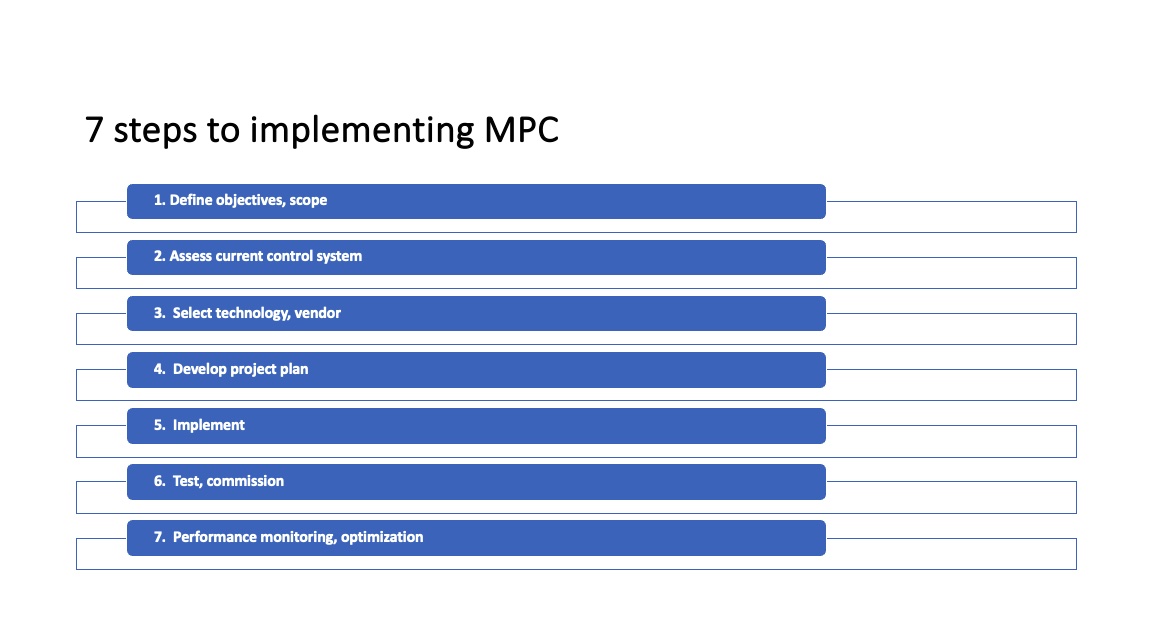
7 Proven Project Steps
Step tests are like the open loop tests in DCS step testing, but run on many variables for days. Plan them with operations.
Poor base level control is the most common reason advanced control fails. Sticky valves, noisy transmitters and bad PID tuning must be fixed first, or the optimiser will fight the base layer.
Horizon and Sample Time Rules
Settling time ≈ Dead time + 4 × Time constant
Prediction horizon P ≈ Settling time ÷ Ts, Control horizon M ≈ 20 percent of P
Example: time constant 20 min, dead time 5 min
Ts = 2 min, settling = 85 min
P ≈ 43 samples, M ≈ 9 moves
These are starting rules of thumb used in MATLAB and textbook guidance. Final values come from simulation and plant testing.
Tuning Calculator
Longer horizons give smoother control but need more computation. Very short horizons make the controller aggressive.
- Handles interactions and dead time.
- Operates close to constraints.
- Higher throughput and lower energy.
- Consistent operation across shifts.
- Model building effort.
- Needs good base control.
- Operator trust and training.
- Models degrade as plants change.
Machine learning models are increasingly used alongside MPC, as discussed in AI in PLC, SCADA and DCS.
Stanford MPC Lecture PDF
Understanding MPC Video
Model Predictive Control FAQ
Related Articles
- PID Controller Types
- What Is Cascade Control
- DCS Control Strategies
- How to Tune a PID Controller
- Digital Twin in Automation
External References
- MPC Lecture, Stanford University
- 7 Ways MPC Benefits Food and Beverage, Control Engineering
- Advanced Process Controls, McKinsey
What We Learn Today
- Model predictive control predicts, optimises and repeats every sample.
- It handles interactions, dead time and constraints better than PID alone.
- Good base control, step tests and maintenance decide success.