A single number on a screen tells an operator where the process is, but only a trend tells where it is heading. Well designed trends turn thousands of stored samples into an early warning that operators can read in a glance.
Trends are the most used troubleshooting tool in any control room, yet many are cluttered, badly scaled or too slow to help. Good SCADA trending design picks the right tags, spans, scales and sample rates so the picture tells the truth.

What Is SCADA Trending?
SCADA trending is the display of process values against time on an operator screen, using either live data from the controllers or stored data from a historian. It lets operators and engineers see the direction, speed and pattern of change, which a single number on a human machine interface cannot show.
A trend is built from pens, where each pen is one tag such as a flow, level or valve output, drawn on a time axis with a value scale. The data comes from the same polling and logging chain described in how SCADA systems work.
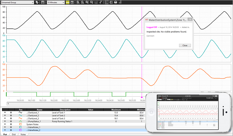
Trihedral describes its VTScada trend viewer as offering a single timeline that covers the entire lifespan of an application, with minimum, maximum and average values and logarithmic scaling. It also lets users export any range of data to a file or database.
Real Time Versus Historical Trends
Plots live values as they arrive from the controller, usually covering minutes to a few hours.
Reads stored values from the historian for any period, from hours to years.
A small trend placed inside a process graphic next to the equipment it describes.
Two periods or two batches drawn on the same axes for comparison.
Real time SCADA trending usually draws from a short memory buffer in the SCADA server, so it is fast but limited in length. Historical SCADA trending draws from a process historian, which can hold years of data but depends on how the values were stored.
Many modern SCADA trending packages blend the two, so a trend scrolls live and the user can simply drag back into history. Behind the scenes the software switches from the live buffer to the archive, as explained for DCS historian data storage.
| Feature | Real Time Trend | Historical Trend |
|---|---|---|
| Data source | Live poll or subscription | Historian archive |
| Typical span | Minutes to hours | Hours to years |
| Resolution | Every poll | As stored after deadband |
| Main user | Operator | Operator, engineer, manager |
| Main risk | Lost on server restart | Detail lost to compression |
An ISA101 committee member writing on Automation.com notes that embedded trends with indications of the desirable range are used in all high performance HMI graphics. The same article says that trend on demand capability works poorly in actual practice.
Anatomy of a Trend: Pens, Scales and Time Spans
The time span, or interval, is the width of the time axis. Schneider Electric Geo SCADA documentation defines the Interval as the amount of time shown on the X axis of a historic trend, and an Offset that sets where that window starts.
In SCADA trending the value scale should normally match the calibrated range of the instrument, for example 0 to 10 bar for a pressure transmitter. Auto scaling looks attractive but magnifies tiny noise into dramatic waves, a problem related to analog signal resolution.
Pens need colours that stay distinct on the background and a legend showing tag name, description, units and current value. Control Engineering reminds designers not to rely on colour as the sole source of information, so line style and labels should also separate pens.
Lock the value scale of each pen to its instrument range on operator trends. Allow auto scale only on engineering analysis screens where the user knows it is switched on.
8 Practical Rules for SCADA Trending
These rules follow the thinking of ANSI/ISA 101.01, the HMI standard for process industries. Our guide on SCADA HMI screen design to ISA 101 explains the display hierarchy into which these trends fit.
Rule eight matters most in everyday SCADA trending. The Automation.com article observes that a typical operator might have about a dozen Level 2 graphics, and each of those should carry its key trends ready to view without hunting for tags.
Sample Rate, Deadband and What You Lose
The sample rate decides how often a value is read, while the deadband decides whether a new value is worth storing. If either is set too coarse, short spikes, valve stick slip and fast oscillations simply do not appear in historical SCADA trending, as discussed in store and forward historians.
A deadband of 0.5 percent of span on a 0 to 10 bar transmitter is 0.05 bar, so any change smaller than that is not stored. The trend then shows a flat line followed by a step, which can hide a slowly hunting loop.
Field devices that report by exception add a second filter at the RTU, as described in report by exception in DNP3. Know every deadband between the transmitter and the trend before trusting the picture.
Samples per Pixel Formula
A SCADA trending window can only draw as many points as it has horizontal pixels. When the samples in view greatly exceed the width, the software must reduce them, and the method it uses decides whether spikes survive.
Samples per pixel = samples in view ÷ trend width (pixels)
Example:
Time span = 60 min = 3600 s, sample interval = 1 s, width = 800 pixels
Samples in view = 3600 ÷ 1 = 3600
Samples per pixel = 3600 ÷ 800 = 4.50
At 4.50 samples per pixel, a good trend draws the minimum and maximum of each group so a short spike is still visible. A trend that plots only one sample per pixel can miss it completely.
Trend Resolution Calculator
Second Worked Example: A Full Shift View
An engineer opens an 8 hour shift trend with the same 1 second samples and 800 pixel width. Samples in view = 28800 ÷ 1 = 28800, and samples per pixel = 28800 ÷ 800 = 36.
Thirty six samples must now share each pixel, so check that the trend uses minimum and maximum reduction. Storage grows too, since 2000 tags at 1 second create 172.8 million values per day, the kind of load covered in SCADA database growing too fast.
Troubleshooting a Plant With SCADA Trending
Valve stiction is one of the most common finds of SCADA trending. Plotting controller output and flow together reveals the classic stick slip shape, which is the first step in any control valve troubleshooting job.
For tuning, trend the setpoint, process value and output on one chart with a span of a few loop periods. This view is essential when following the method in how to tune a PID controller.
Simultaneous gaps on every tag from one station point to communications rather than the process. Check the steps in SCADA communication problems before blaming the instruments.
When comparing an event on two servers, first confirm both clocks agree. A trend that is a few seconds off can make an effect appear before its cause.
Common SCADA Trending Mistakes
Time stamps are another hidden trap. When servers, controllers and RTUs disagree on time, overlays mislead, which is why SCADA time synchronization matters for every trend.
In 2009 the Electric Power Research Institute ran a major test of high performance HMI concepts, according to Automation.com. Graphics with embedded trends and clear range indications were part of the approach tested.
Design Checklist for Operator Trends
- Each key graphic has preconfigured trends for its main values.
- Every pen shows tag, description, units and current value.
- Scales match calibrated instrument ranges.
- Normal operating bands are shaded or marked.
- Time spans suit the speed of each process.
- Sample rate and deadband reveal real disturbances.
- Server and controller clocks are synchronized.
- Trend data can be exported for analysis.
Review this SCADA trending checklist with operators, not only with engineers, because they use the trends every shift. Pair it with sound alarm management to ISA 18.2, since a good trend often explains why an alarm appeared.
Finally, keep tag names and descriptions consistent with your SCADA tag database design. A trend legend that reads FT101 PV with no description slows down every investigation.
- Early warning of drifting or abnormal values.
- Fast root cause analysis after trips.
- Clear evidence for tuning and valve problems.
- Shared picture for operators and engineers.
- Deadband and compression hide small changes.
- Large spans need data reduction on screen.
- Poor scales and colours mislead users.
- Historian storage grows with fast sampling.
Human System Interface Guidelines PDF
Trend and History Tutorial Video
SCADA Trending FAQ
It is the display of process values against time on an operator screen. The data comes either live from controllers or from a historian archive.
Trends show direction, speed and pattern of change that a single number cannot. Operators use them to spot trouble early, and engineers use them to find the cause of a trip.
A real time trend plots live values from a short memory buffer, usually covering minutes to hours. A historical trend reads stored data from the historian for any period.
Real time views are fast but short lived. Historical views go back years, but they only show what the historian actually stored after deadband and compression.
Good SCADA trending keeps each chart to a small group of related pens that answer one question. A controller trend, for example, needs setpoint, process value and controller output.
Crowded trends with ten or more lines make the important line hard to find. If you need more values, create a second trend with its own purpose and title.
In SCADA trending, a fixed scale matched to the instrument range shows the true size of a change. Operators learn what normal looks like and spot deviations quickly.
Auto scale magnifies noise and changes whenever the data changes. It is useful for engineering analysis but confusing on the everyday operator displays used in every shift.
A historian with a deadband stores a new value only when it moves more than the set amount. Smaller changes are simply discarded to save disk space on the server.
Historical SCADA trending then shows flat lines and steps instead of the real signal. Choose a deadband small enough to show the disturbances that matter for that loop.
For SCADA trending, match the sample rate to the speed of the process and the purpose of the trend. Fast flow and pressure loops often need sampling every second or faster.
Slow tank levels and furnace temperatures can be sampled much less often. Always check that the chosen rate still captures the shortest event you need to investigate.
Yes, it is one of the most useful checks that SCADA trending offers. Plot controller output and the measured flow together over a few minutes.
A sticking valve shows output ramping while flow stays flat, followed by a sudden jump in flow. This stick slip shape is a strong sign that the valve needs maintenance.
Related Articles
- SCADA HMI Screen Design to ISA 101
- What Is a Process Historian
- DCS Historian Explained
- SCADA Time Synchronization With NTP and PTP
- Control Valve Troubleshooting
External References
- NUREG 0700 Rev 3, Human System Interface Design Review Guidelines, US NRC
- The High Performance HMI, Automation.com
- SCADA, Wikipedia
What We Learn Today
- SCADA trending plots process values against time from live buffers or a historian, showing the direction and speed of change that a single number cannot reveal.
- Fix pen scales to instrument ranges, shade the normal band, keep pens few and build trends into graphics instead of relying on trend on demand.
- Sample rate and historian deadband decide which spikes survive, and samples per pixel equals time span divided by sample interval and trend width.