
Before understanding zero and span concept, let us first understand linearity. The main goal of calibration is to make sure an instrument’s input and output match each other correctly across its full operating range. This relationship is often shown using a graph that compares the input to the output.
For most industrial instruments, this graph appears as a straight line, meaning the instrument responds in a linear way.
Table of Contents
ToggleZero and Span Adjustments
This graph 1 shows how any percentage of input should match the same percentage of output, consistently from 0% up to 100%.
Things get a bit more detailed when the axes are labeled with actual measurement units instead of just percentages.
For example, consider a pressure transmitter. Its job is to detect fluid pressure and provide an electronic signal that represents that pressure.
In this case, the graph might show an input range of 0 to 100 pounds per square inch (PSI) and an output range of 4 to 20 milliamps (mA) of electric current.
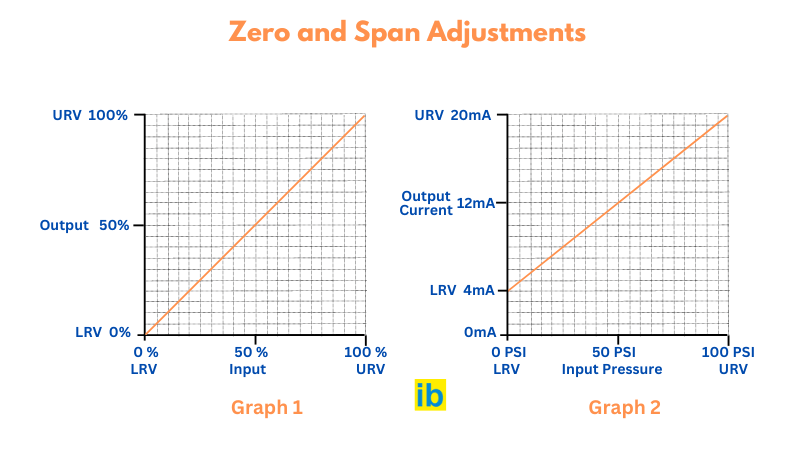
Please see Graph 2. Even though the graph is linear, notice that zero pressure does not mean zero current. This is known as a live zero because the 0% measurement point (0 PSI pressure) corresponds to a small but non-zero output signal.
In this case, 0 PSI is the transmitter’s Lower Range Value (LRV) on the input side, but the LRV on the output side is 4 mA rather than 0 mA.
Like any straight-line relationship, this behavior can be described using the familiar slope-intercept equation.
Linear Slope Intercept Equation for Instrument Calibration
y = mx + b
Where,
y = Vertical Position on Graph
x = Horizontal Position on Graph
m = Slope of Line
b = Point of Intersection between Line & Vertical y Axis
Suppose,
x = Input Pressure in units of PSI
y = Output current in units of mA
We can write the equation for this instrument as below
y=0.16x + 4
On the actual device (the pressure transmitter), there are two settings that allow us to align the instrument’s response with the ideal equation. One setting is called the zero, and the other is called the span. These two settings directly relate to the b and m terms in the linear function: the zero adjustment shifts the instrument’s curve up or down on the graph (b), while the span adjustment alters the slope of the curve on the graph (m). By fine-tuning both zero and span, we can configure the instrument to cover any measurement range within the manufacturer’s specifications.
The connection between the slope-intercept equation and an instrument’s zero and span adjustments also explains how these corrections are made inside any instrument.
A zero adjustment is achieved by adding or subtracting a certain value, just as the y-intercept term b adds or subtracts in the equation mx.
A span adjustment is always achieved by multiplying or dividing a value, just as the slope m multiplies the input variable x.
Zero and Span Calibration
Zero Adjustments
Instruments often include zero adjustments, which can be achieved in several ways, such as:
- Applying a bias force (using a spring or weight to shift a mechanism)
- Introducing a mechanical offset (adding or removing a small amount of movement)
- Applying a bias voltage (adding or subtracting a fixed amount of electrical potential)
Span Adjustments
Span adjustments, on the other hand, are typically carried out through methods like:
- Changing the fulcrum position of a lever to alter force or motion multiplication
- Adjusting the amplifier gain to multiply or divide a voltage signal
- Modifying the spring rate, which changes the force per unit of stretch or compression
Interaction Between Zero and Span
It’s important to note that in most analog instruments, zero and span adjustments are not independent — they interact. In particular, altering the span often shifts the zero point. Because of this, calibrating such instruments can be more time-consuming. The technician must go back and forth between adjusting the lower range (zero) and the upper range (span) until both are set accurately.
What we learn today?
Most industrial instruments are designed to provide a linear output, meaning the output signal increases or decreases at a steady rate as the input value changes.
The zero adjustment sets the output level when the input is at 0%, or at its lowest range value (LRV). For instance, in a 4–20 mA loop, the output will be 4 mA when the input is at 0%.
The span adjustment defines the entire range of output from the lowest point to the highest. Using the same 4–20 mA example, the span equals 16 mA (20 mA – 4 mA).


I hope you like above blog. There is no cost associated in sharing the article in your social media. Thanks for reading!! Happy Learning!!